1 图片读取与通道
图片读取后,默认是个numpy的3维数组(row行数是height, col高度是图片宽度,3是BGR通道)
import cv2
img1 = cv2.imread('./dog_backpack.png')
img1.shape
(1401, 934, 3)
注意上面通道顺序是BGR哦,反人类吧,需要做转换,才能正常显示图片,如下:
img1 = cv2.cvtColor(img1, cv2.COLOR_BGR2RGB)

import matplotlib.pyplot as plt
plt.imshow(img)
调整图片尺寸(硬调)
img1 = cv2.resize(img1, (1200, 1200))
根据百分比调整的api有点反人类,建议用ratio计算后调用上面的
2 如何给窗口设置回调
# Create a named window for connections
cv2.namedWindow('Test')

# Bind draw_rectangle function to mouse cliks
cv2.setMouseCallback('Test', draw_circle)

def draw_circle(event,x,y,flags,param):

    global center,clicked

    # get mouse click on down and track center
    if event == cv2.EVENT_LBUTTONDOWN:
        center = (x, y)
        clicked = False

    # Use boolean variable to track if the mouse has been released
    if event == cv2.EVENT_LBUTTONUP:
        clicked = True
3 图形绘制
4 图片混合(Blending)和叠加(Paste)
只有相同尺寸的图才能Blending,效果如下图:
blended = cv2.addWeighted(src1=img1, alpha=0.7, src2=img2, beta=0.3, gamma=0)
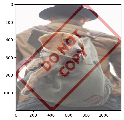
不相同尺寸图片,可以先构造与大图片相同的空图片,把小图放上去,两张图做blend
import cv2
import numpy as np
import matplotlib.pyplot as plt

img1 = cv2.imread('dog_backpack.png')
img2 = cv2.imread('watermark_no_copy.png')

img1 = cv2.cvtColor(img1, cv2.COLOR_BGR2RGB)
img2 = cv2.cvtColor(img2, cv2.COLOR_BGR2RGB)
img2 = cv2.resize(img2, (640, 640))

# make a new img of big size
img_new = np.ones(img1.shape, dtype=np.uint8) * 255
# set small to new big size
img_new[0:img2.shape[0], 0:img2.shape[1],:] = img2

# blended same size
blended = cv2.addWeighted(src1=img1,alpha=0.7,src2=img_new,beta=0.3,gamma=0)
plt.imshow(blended)
效果:

5 阈值(Threshold)处理
可以在灰度图的基础上,做阈值(Threshold)处理,可以得到对比度不同的图,这个在很多场景很有用:
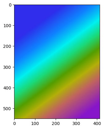
img = cv2.imread('./rainbow.jpg', 0)
th, th_img = cv2.threshold(img, 127, 255, cv2.THRESH_BINARY)
plt.imshow(th_img, cmap='gray')
效果如下图:
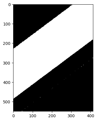
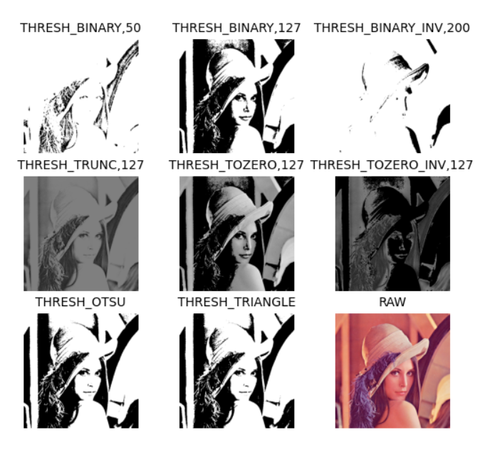
参数还可以用THRESH_BINARY_INV(黑白反)、THRESH_TRUNC(大于th截断,小于的不变)、THRESH_TOZERO(大于th不变,小于设成0)、THRESH_TOZERO_INV(大于设成0,小于不变)
此外,上述与参数还可以 逻辑或 cv2.THRESH_OTSU、cv2.THRESH_TRIANGLE两个自动选择阀值的参数(此时需保证参数的阀值为0)
效果可以参考:
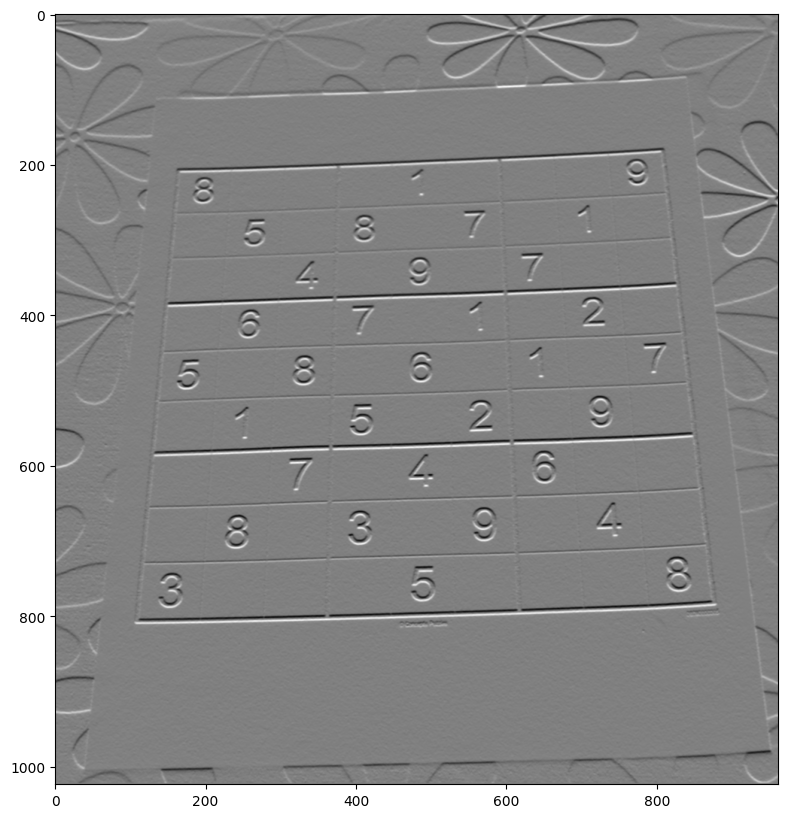
6 模糊(Blur)、平滑(Smooth)
主要用于去除图片噪声,保留主要细节。
没太get到这俩的区别,都有很多实现方法
不同kernel在线效果网站:Image Kernels
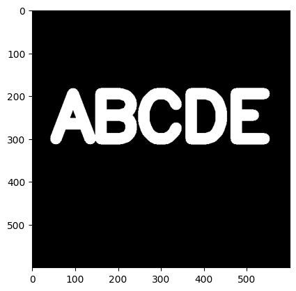
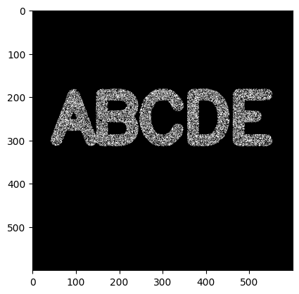
原始图

使用2D核过滤,可以发现边缘模糊了,空心字变实了
kernel = np.ones(shape=(5,5), dtype=np.float32) / 25
img_filter = cv2.filter2D(img, -1, kernel)

使用cv内置模糊blur:
img_filter = cv2.blur(img, ksize=(5,5))

高斯模糊:
img_filter = cv2.GaussianBlur(img, (5,5), 10)
中值模糊:
img_filter = cv2.medianBlur(img, 7)
双边滤波(Bilateral Filtering):
img_filter = cv2.bilateralFilter(img,9,75,75)

7 使用均值模糊(Median Blur)去噪声
均值模糊的主要用途,其实是去除噪声:
先给图加点噪点:
 修复后:
修复后:
img_fix = cv2.medianBlur(img, 5)

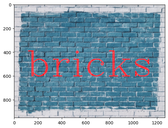
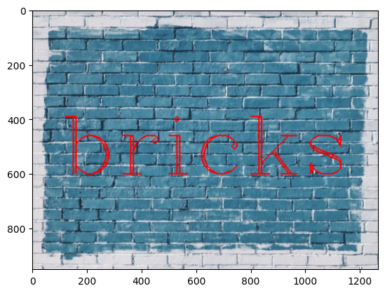
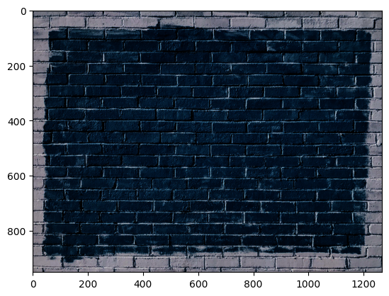
8 伽玛校正
原始图
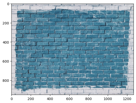
注意:所有变换前,都需要把0~255弄到0~1之间,方便变换,变换完成后,其实是需要转会0~255的,但是plt的imshow能兼容识别0~1。
使用伽玛校正(Gamma Correction) 提升亮度:
import cv2
import numpy as np
import matplotlib.pyplot as plt

img = cv2.imread('./bricks.jpg').astype(np.float32) / 255
img = cv2.cvtColor(img, cv2.COLOR_BGR2RGB)

gamma = 1/4
img_gamma = np.power(img, gamma)

plt.imshow(img_gamma)
gamma参数小于1变亮
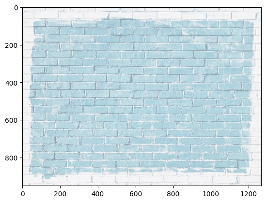
gamma参数大于1变暗
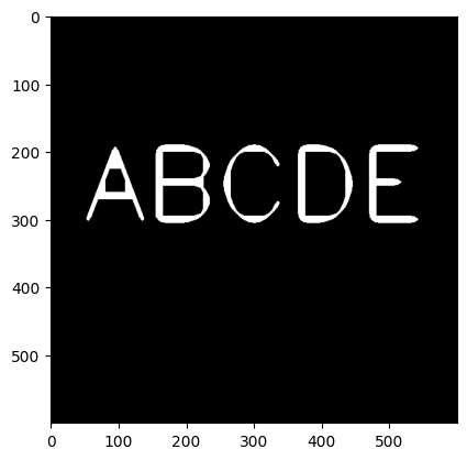
9 Erosion(腐蚀)
腐蚀(erosion)用于提取图像的边缘
原图:
腐蚀操作,直接这里kernel和iteration都会影响'腐蚀'的效果:
kernel = np.ones((5,5), np.uint8)
erosion_img = cv2.erode(img, kernel, iterations=4)

plt.imshow(erosion_img, cmap='gray')
10 形态学(Morphological Operators)操作之开运算(Open)去除随机噪声
先加一些随机噪声:
white_noise = np.random.randint(low=0, high=2, size=(600,600))
white_noise = white_noise * 255

noise_img = white_noise + img
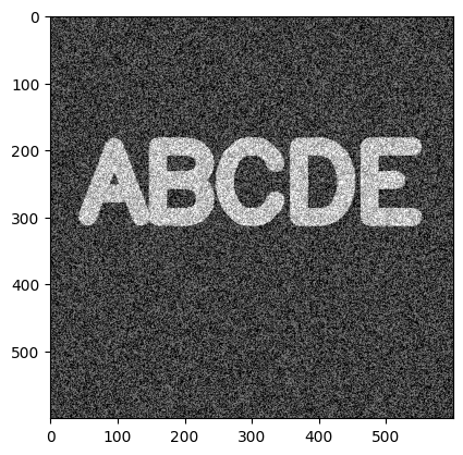
使用形态学(Morphological)开运算(Open)处理,去处图像中孤立的随机噪声,其原理是先腐蚀再膨胀:
kernel = np.ones((5,5),np.uint8)
open_img = cv2.morphologyEx(noise_img, cv2.MORPH_OPEN, kernel)
plt.imshow(open_img, cmap='gray')

11 形态学(Morphological Operators)操作之闭运算(Close)去除前景噪声
现在增加难度,只给前景(ABCDE)增加随机黑色噪声
black_noise = np.random.randint(low=0,high=2,size=(600,600))
black_noise= black_noise * -255
noise_img = black_noise + img
noise_img[noise_img==-255] = 0
此时再用OPEN方法,就会发现,整个都被摸掉了,需要用Close方法,原理是先扩张再腐蚀:
kernel = np.ones((5,5),np.uint8)
open_img = cv2.morphologyEx(noise_img, cv2.MORPH_CLOSE, kernel)
plt.imshow(open_img, cmap='gray')

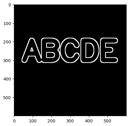
12 形态学(Morphological Operators)操作之梯度(Gradient)
形态学梯度(Gradient)是膨胀与腐蚀(Erosion)的差值,用于刻画目标边界 或 边缘位于图形灰度级别剧烈变化的区域,突出高亮区域的外围,如下(图片使用无噪声的初始版本):
kernel = np.ones((5,5),np.uint8)
g_img = cv2.morphologyEx(img, cv2.MORPH_GRADIENT, kernel)
plt.imshow(g_img, cmap='gray')
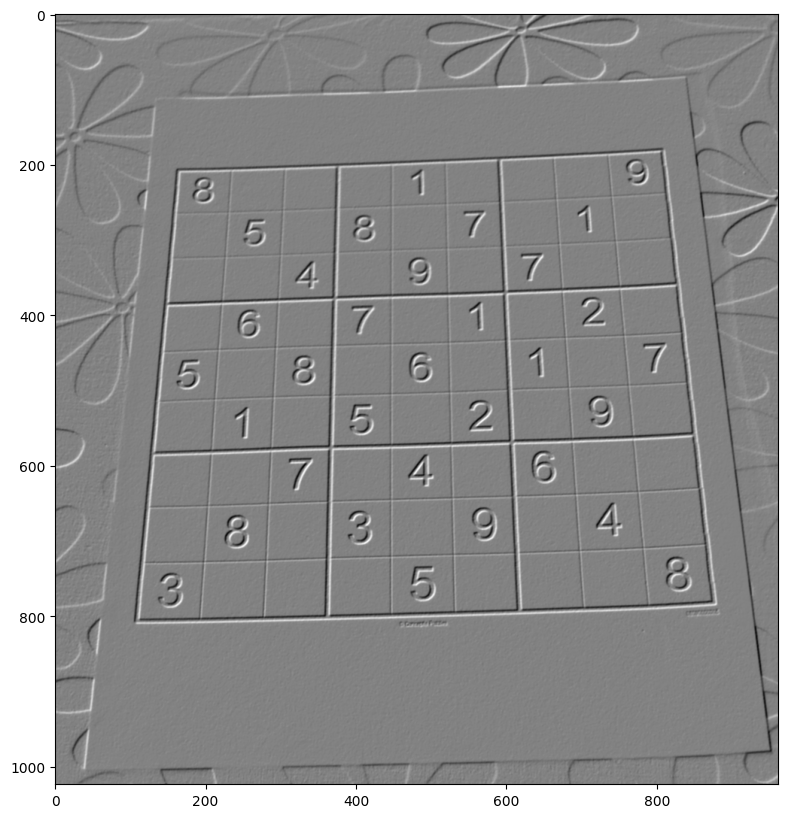
13 索贝尔算子(Sobel)、Laplacian算子提取边缘
原图:
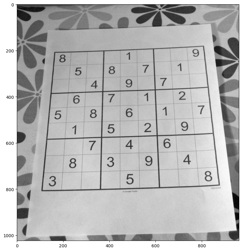
索贝尔算子,提取边缘,可以用第3、4个参数控制横向和纵向
img_sobelx = cv2.Sobel(img, cv2.CV_64F,1,0,ksize=5)
img_sobely = cv2.Sobel(img, cv2.CV_64F,0,1,ksize=5)
img_sobel = cv2.Sobel(img, cv2.CV_64F,1,1,ksize=5)
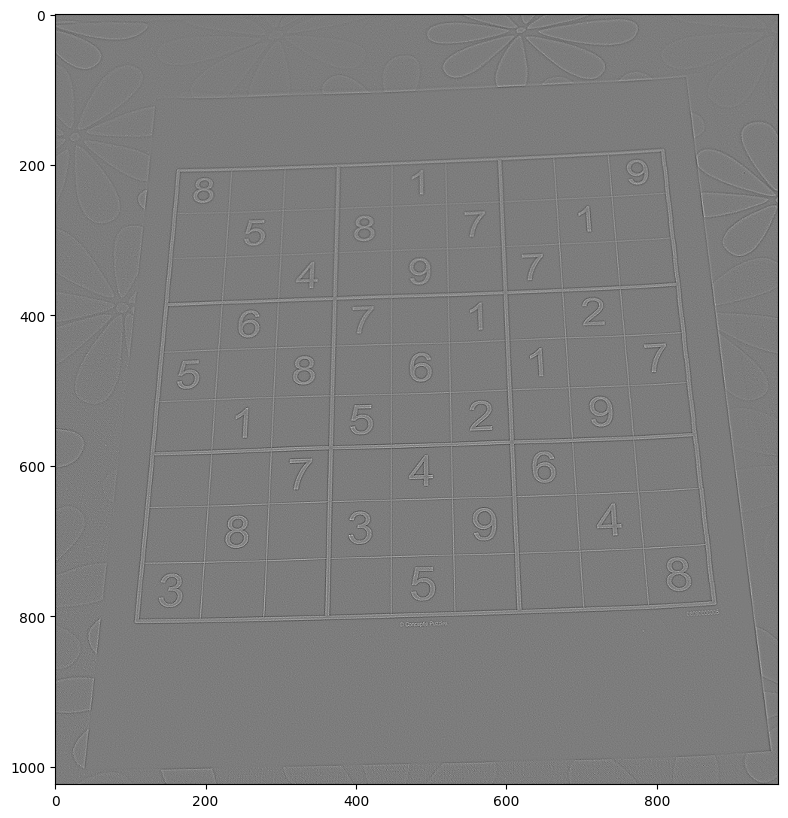
以下3个图分别是,横向、纵向、横纵的:
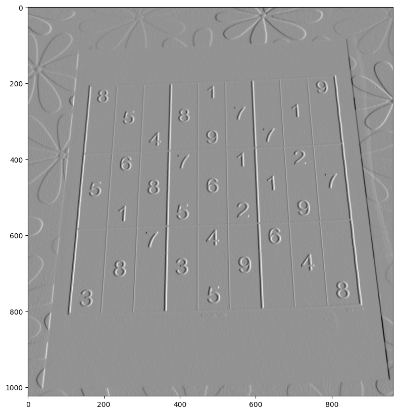

可以发现最后的这个,反而不如x和y的,可以对这俩做叠加(Blending):
img_sobelx = cv2.Sobel(img, cv2.CV_64F,1,0,ksize=5)
img_sobely = cv2.Sobel(img, cv2.CV_64F,0,1,ksize=5)
img_blended = cv2.addWeighted(src1=img_sobelx,alpha=0.5,src2=img_sobely,beta=0.5,gamma=0)
也可以用Laplacian算子:
img_lap = cv2.Laplacian(img,cv2.CV_64F)
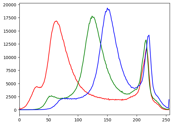
14 计算图片的直方图
单通道R:
hist_values = cv2.calcHist([bricks_img], channels=[0], mask=None, histSize=[256], ranges=[0,256])
绘制3个通道的,注意我这里转成rgb了:
bricks_img = cv2.imread('./bricks.jpg')
bricks_img = cv2.cvtColor(bricks_img, cv2.COLOR_BGR2RGB)


img = bricks_img

color = ('r', 'g', 'b')

for i, col in enumerate(color):
  histr = cv2.calcHist([img], [i], None, [256], [0,256])
  plt.plot(histr,color = col)
  plt.xlim([0,256])

plt.show()
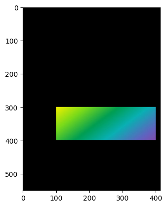
15 遮罩
img = rainbow_img

mask = np.zeros(img.shape[:2], np.uint8)
mask.shape
mask[300:400, 100:400] = 255

masked_img = cv2.bitwise_and(img, img, mask = mask)
plt.imshow(masked_img)
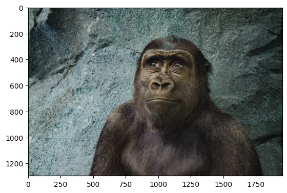
16 利用hsv通道的均值化(equalize)提高对比度
hsv的v通道一般是亮度,我们单独对它做均值话,可以提高图片整体亮度
原图
import cv2
import matplotlib.pyplot as plt
img_gorilla = cv2.imread('./gorilla.jpg')
img_gorilla_hsv = cv2.cvtColor(img_gorilla, cv2.COLOR_RGB2HSV)
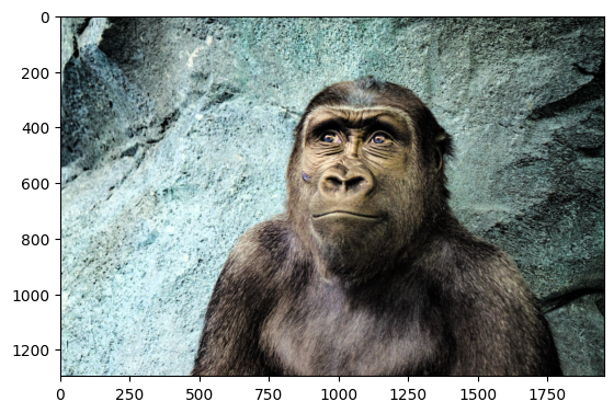
img_gorilla_hsv[:,:,2] = cv2.equalizeHist(img_gorilla_hsv[:,:,2])
img_gorilla_new = cv2.cvtColor(img_gorilla_hsv, cv2.COLOR_HSV2RGB)
plt.imshow(img_gorilla_new)
效果
17 打开摄像头并绘制桢
import cv2

cap = cv2.VideoCapture(0)


# 获取设备长宽
width = int(cap.get(cv2.CAP_PROP_FRAME_WIDTH))
height = int(cap.get(cv2.CAP_PROP_FRAME_HEIGHT))

# 计算坐标并保持是int
x = width//2
y = height//2

# Width and height
w = width//4
h = height//4

while True:
    # 绘制帧
    ret, frame = cap.read()

    # Draw a rectangle on stream

    cv2.rectangle(frame, (x, y), (x+w, y+h), color=(0,0,255),thickness= 4)

    # Display the resulting frame
    cv2.imshow('frame', frame)

   # This command let's us quit with the "q" button on a keyboard.
    # Simply pressing X on the window won't work!
    if cv2.waitKey(1) & 0xFF == ord('q'):
        break

# When everything is done, release the capture
cap.release()
cv2.destroyAllWindows()
18 打开视频并绘制桢
注意这里速度要按照fps做一下等待,否则速度过快
import cv2
import time
# Same command function as streaming, its just now we pass in the file path, nice!
cap = cv2.VideoCapture('../DATA/video_capture.mp4')

# FRAMES PER SECOND FOR VIDEO
fps = 25

# Always a good idea to check if the video was acutally there
# If you get an error at thsi step, triple check your file path!!
if cap.isOpened()== False:
    print("Error opening the video file. Please double check your file path for typos. Or move the movie file to the same location as this script/notebook")


# While the video is opened
while cap.isOpened():


    # Read the video file.
    ret, frame = cap.read()

    # If we got frames, show them.
    if ret == True:


        # 解决速度过快问题
        time.sleep(1/fps)
        cv2.imshow('frame',frame)

        # Press q to quit
        if cv2.waitKey(25) & 0xFF == ord('q'):

            break

    # Or automatically break this whole loop if the video is over.
    else:
        break

cap.release()
# Closes all the frames
cv2.destroyAllWindows()
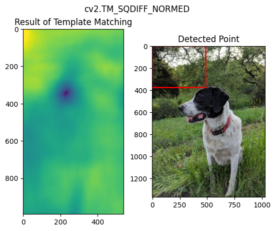
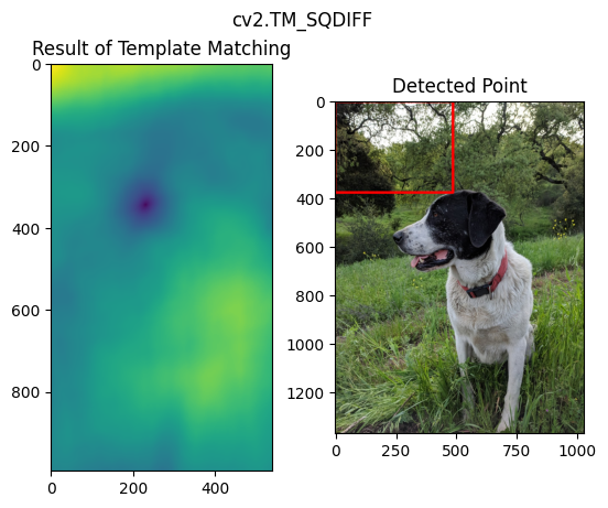
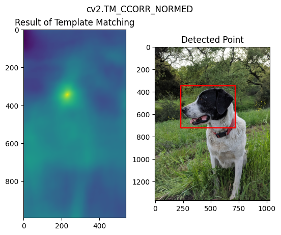
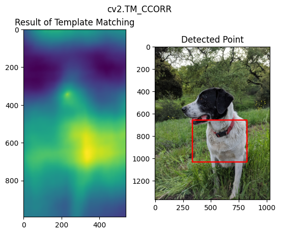
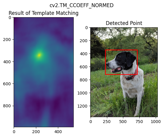
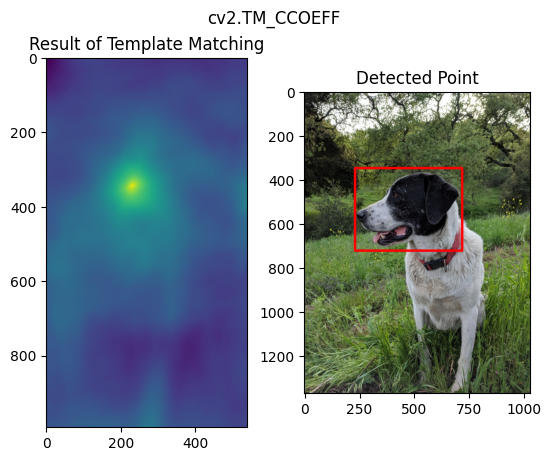
18 目标检测之模板匹配(Template Matching)
用于目标是大图的一部分的情况,最简单的case。
import cv2
import matplotlib.pyplot as plt

full = cv2.imread('./sammy.jpg')
full = cv2.cvtColor(full, cv2.COLOR_BGR2RGB)

face = cv2.imread('./sammy_face.jpg')
face = cv2.cvtColor(face, cv2.COLOR_BGR2RGB)
height, width, channels = face.shape

methods = ['cv2.TM_CCOEFF', 'cv2.TM_CCOEFF_NORMED', 'cv2.TM_CCORR','cv2.TM_CCORR_NORMED', 'cv2.TM_SQDIFF', 'cv2.TM_SQDIFF_NORMED']

for m in methods:
  full_copy = full.copy()

  method = eval(m)
  res = cv2.matchTemplate(full_copy, face, method)

  min_val, max_val, min_loc, max_loc = cv2.minMaxLoc(res)

  if m in [cv2.TM_SQDIFF, cv2.TM_SQDIFF_NORMED]:
      top_left = min_loc
  else:
      top_left = max_loc

  bottom_right = (top_left[0] + width, top_left[1] + height)
  cv2.rectangle(full_copy,top_left, bottom_right, 255, 10)

  # plt
  plt.subplot(121)
  plt.imshow(res)
  plt.title('Result of Template Matching')

  plt.subplot(122)
  plt.imshow(full_copy)
  plt.title('Detected Point')
  plt.suptitle(m)

  plt.show()
不同方法的效果如下:
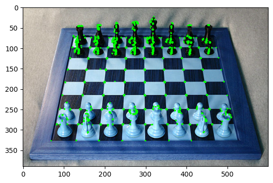
19 角点检测(Corner Detection)
Harris算法
import cv2
import matplotlib.pyplot as plt

chess = cv2.imread('flat_chessboard.png')
chess_gray = cv2.cvtColor(chess, cv2.COLOR_BGR2GRAY)

dst = cv2.cornerHarris(src=chess_gray, blockSize=2, ksize=3, k=0.04)
dst = cv2.dilate(dst, None)

chess[dst>0.01*dst.max()] = [0, 255, 0]

plt.imshow(chess, cmap='gray')
import cv2
import matplotlib.pyplot as plt
import numpy as np
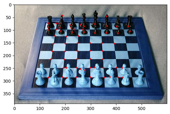
chess = cv2.imread('real_chessboard.jpg')
chess_gray = cv2.cvtColor(chess, cv2.COLOR_BGR2GRAY)
# 64 is how many best corner try to find
corners = cv2.goodFeaturesToTrack(chess_gray,64,0.01,10)
corners = np.int0(corners) # convert np arr to int
for i in corners:
x,y = i.ravel()
cv2.circle(chess,(x,y),3,255,-1)
plt.imshow(chess, cmap='gray')
20 边缘检测(Edge Detection)
import cv2
import matplotlib.pyplot as plt

img = cv2.imread('./sammy_face.jpg')

# best threshold for canny
median_val = np.median(img)
lower = int(max(0, 0.7 * median_val))
upper = int(max(255, 1.3 * median_val))

# blur & canny
blur_img = cv2.blur(img, ksize=(4,4))
edges = cv2.Canny(image=blur_img, threshold1=lower , threshold2=upper)

plt.imshow(edges)
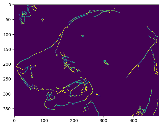
其他算法如前面提过的Sobel、Laplacian也能用。会粗一些。
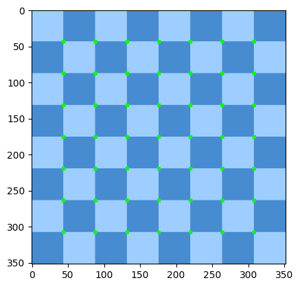
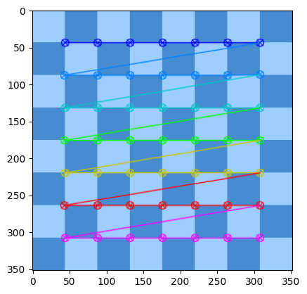
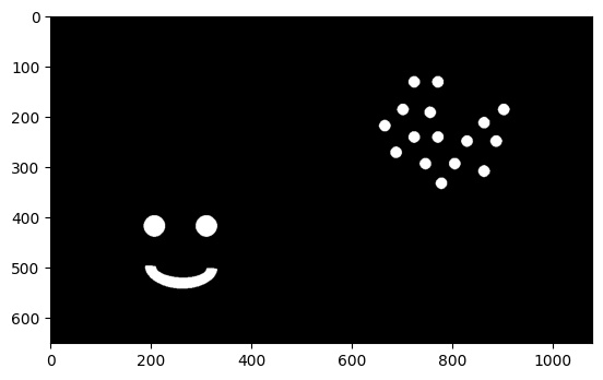
21 网格检测(Grid Detection)
Grid detection(网格检测)是指在图像中检测出网格的位置和大小。这个技术通常用于计算机视觉和机器人视觉中,例如在相机标定和姿态估计中。在相机标定中,我们需要知道相机的内部参数和外部参数,以便将图像中的像素坐标转换为真实世界中的坐标。为了计算这些参数,我们需要在图像中检测出一个已知大小的网格,并使用它来计算相机的畸变和投影矩阵。一部分Grid Detection是用前面讲过的角点检查算法实现的。
import cv2
import matplotlib.pyplot as plt

flat_chess = cv2.imread('./flat_chessboard.png')
found, corners = cv2.findChessboardCorners(flat_chess,(7,7))

if found:
  flat_chess_copy = flat_chess.copy()
  cv2.drawChessboardCorners(flat_chess_copy, (7, 7), corners, found)
  plt.imshow(flat_chess_copy)
else:
    print("OpenCV did not find corners. Double check your patternSize.")
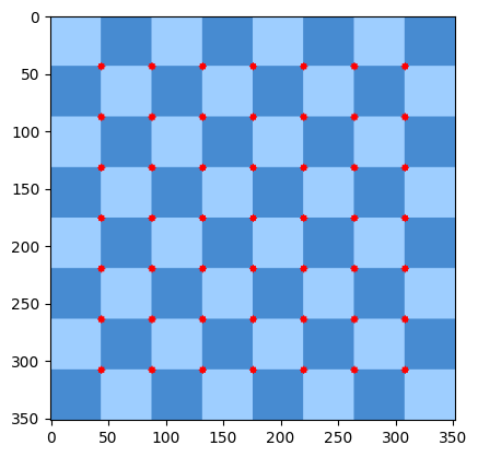
圆形网格检测:
import cv2
import matplotlib.pyplot as plt

dots = cv2.imread('./dot_grid.png')
found, corners = cv2.findCirclesGrid(dots, (10,10), cv2.CALIB_CB_SYMMETRIC_GRID)

dbg_image_circles = dots.copy()
cv2.drawChessboardCorners(dbg_image_circles, (10, 10), corners, found)

plt.imshow(dbg_image_circles)

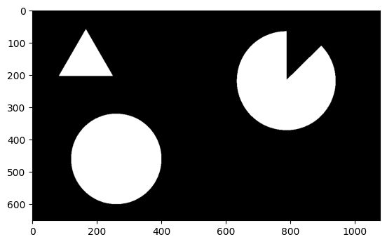
22 轮廓检测(Contour Detection)
Contour Detection(轮廓检测)是一种在计算机视觉中用于检测图像中物体边界的技术。轮廓是连接物体边界上所有连续点的曲线,这些点具有相同的颜色或强度。轮廓检测在许多计算机视觉应用中都很有用,例如目标识别、图像分割和形状分析。
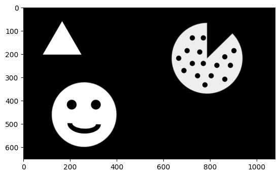
- 下面代码中的RETR_CCOMP是内外轮廓都要,RETR_EXTERNAL是之要外轮廓,还有RETR_TREE / RETR_LIST可选。
- 数组最后一个值-1 / 0 / 1 / 4是分组,这里的-1是外轮廓
import cv2
import numpy as np
import matplotlib.pyplot as plt

img = cv2.imread('./internal_external.png',0)

contours, hierarchy = cv2.findContours(img, cv2.RETR_CCOMP, cv2.CHAIN_APPROX_SIMPLE)

# Set up empty array
external_contours = np.zeros(img.shape)

# For every entry in contours
for i in range(len(contours)):

    # last column in the array is -1 if an external contour (no contours inside of it)
    if hierarchy[0][i][3] == -1:

        # We can now draw the external contours from the list of contours
        cv2.drawContours(external_contours, contours, i, 255, -1)

plt.imshow(external_contours,cmap='gray')
换成 != -1,则是内轮廓:
if hierarchy[0][i][3] != -1:
23 根据轮廓检测绘制外框,合并父子结构
在边缘检测的基础上,还可以利用父子结构,进行简单合并,只保留最大的
img_gray = cv2.cvtColor(img, cv2.COLOR_BGR2GRAY)


edges = cv2.Canny(img_gray, 100, 300)
contours, hierarchy = cv2.findContours(edges, cv2.RETR_TREE, cv2.CHAIN_APPROX_SIMPLE)

merged_contours = []
for i, c in enumerate(contours):
    if hierarchy[0][i][3] == -1:
        merged_contours.append(c)
    else:
        merged_contours[-1] = cv2.convexHull(np.concatenate((merged_contours[-1], c)))

cv2.drawContours(img, merged_contours, -1, (0, 255, 0), 2)

cv2_imshow(img)
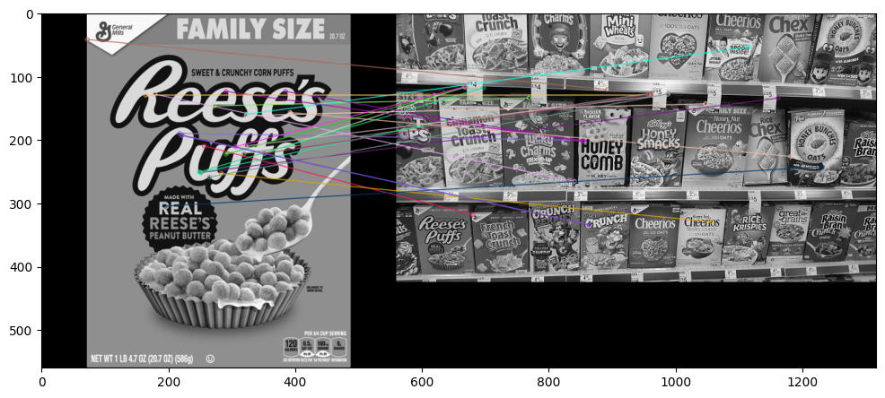
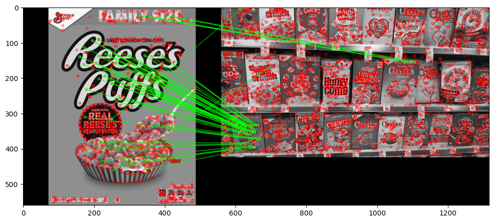
24 特征匹配(Feature Matching)
"特征匹配"(Feature Matching),是计算机视觉中的一种技术,用于在两个或多个图像中找到相同的特征点,并将它们匹配起来。特征匹配在很多计算机视觉应用中都有广泛的应用,例如图像拼接、物体识别和跟踪等。
ORB特征匹配:
效果不好,
import cv2
import numpy as np
import matplotlib.pyplot as plt

def display(img,cmap='gray'):
    fig = plt.figure(figsize=(12,10))
    ax = fig.add_subplot(111)
    ax.imshow(img,cmap='gray')

img1 = cv2.imread('./reeses_puffs.png',0)
img2 = cv2.imread('./many_cereals.jpg',0)

# Initiate ORB detector
orb = cv2.ORB_create()

# find the keypoints and descriptors with ORB
kp1, des1 = orb.detectAndCompute(img1,None)
kp2, des2 = orb.detectAndCompute(img2,None)

# create BFMatcher object
bf = cv2.BFMatcher(cv2.NORM_HAMMING, crossCheck=True)

# Match descriptors.
matches = bf.match(des1,des2)

# Sort them in the order of their distance.
matches = sorted(matches, key = lambda x:x.distance)

# Draw first 25 matches.
img_matches = cv2.drawMatches(img1,kp1,img2,kp2,matches[:25],None,flags=2)

display(img_matches)
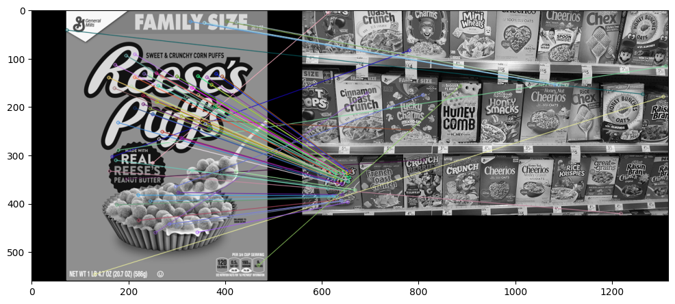
SIFT特征:
效果较好,发现大部分特征都匹配到了对的图上
import cv2
import numpy as np
import matplotlib.pyplot as plt

def display(img,cmap='gray'):
    fig = plt.figure(figsize=(12,10))
    ax = fig.add_subplot(111)
    ax.imshow(img,cmap='gray')

img1 = cv2.imread('./reeses_puffs.png',0)
img2 = cv2.imread('./many_cereals.jpg',0)

# Create SIFT Object
sift = cv2.xfeatures2d.SIFT_create()

# find the keypoints and descriptors with SIFT
kp1, des1 = sift.detectAndCompute(img1,None)
kp2, des2 = sift.detectAndCompute(img2,None)

# BFMatcher with default params
bf = cv2.BFMatcher()
matches = bf.knnMatch(des1,des2, k=2)

# Apply ratio test
good = []
for match1,match2 in matches:
    if match1.distance < 0.75*match2.distance:
        good.append([match1])

# cv2.drawMatchesKnn expects list of lists as matches.
img_matches = cv2.drawMatchesKnn(img1,kp1,img2,kp2,good,None,flags=2)

display(img_matches)
上面两个搜索都是基于bf(暴力的),速度有些慢,我们可以换一个匹配方法,例如flann的:
这里不止画了最佳match,把特征也画出来了(红点)
import cv2
import numpy as np
import matplotlib.pyplot as plt

def display(img,cmap='gray'):
    fig = plt.figure(figsize=(12,10))
    ax = fig.add_subplot(111)
    ax.imshow(img,cmap='gray')

img1 = cv2.imread('./reeses_puffs.png',0)
img2 = cv2.imread('./many_cereals.jpg',0)

# Initiate SIFT detector
sift = cv2.xfeatures2d.SIFT_create()

# find the keypoints and descriptors with SIFT
kp1, des1 = sift.detectAndCompute(img1,None)
kp2, des2 = sift.detectAndCompute(img2,None)

# FLANN parameters
FLANN_INDEX_KDTREE = 0
index_params = dict(algorithm = FLANN_INDEX_KDTREE, trees = 5)
search_params = dict(checks=50)

flann = cv2.FlannBasedMatcher(index_params,search_params)

matches = flann.knnMatch(des1,des2,k=2)

# Need to draw only good matches, so create a mask
matchesMask = [[0,0] for i in range(len(matches))]

# ratio test
for i,(match1,match2) in enumerate(matches):
    if match1.distance < 0.7*match2.distance:
        matchesMask[i]=[1,0]

draw_params = dict(matchColor = (0,255,0),
                   singlePointColor = (255,0,0),
                   matchesMask = matchesMask,
                   flags = 0)

img_matches = cv2.drawMatchesKnn(img1,kp1,img2,kp2,matches,None,**draw_params)

display(img_matches)
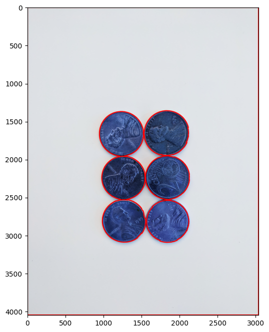
25 分水岭算法(Watershed Algorithm)
Watershed Algorithm(分水岭算法)是一种图像分割算法,主要用于将图像分割成多个区域。它可以将图像中的每个像素视为地形表面上的一个点,并将这些点视为水滴。当水滴落在山峰上时,它会沿着山峰的边缘流动,直到到达山谷。在图像中,山峰表示图像中的物体,而山谷表示物体之间的边界。通过将每个像素视为水滴并模拟水滴的流动,Watershed Algorithm可以将图像分割成多个区域,每个区域代表一个物体。Watershed Algorithm在计算机视觉和图像处理领域有广泛的应用,例如图像分割、目标检测、图像分析等。
在下面的例子中,首先找到明确是前景的点,然后再用分水岭算法
import numpy as np
import cv2
import matplotlib.pyplot as plt

def display(img,cmap=None):
    fig = plt.figure(figsize=(10,8))
    ax = fig.add_subplot(111)
    ax.imshow(img,cmap=cmap)

img_coins = cv2.imread('./pennies.jpg')
# blur
img_coins_blur = cv2.medianBlur(img_coins, 35)
# threshold adaptive
img_coins_gray = cv2.cvtColor(img_coins_blur,cv2.COLOR_BGR2GRAY)
ret, thresh = cv2.threshold(img_coins_gray,0,255,cv2.THRESH_BINARY_INV+cv2.THRESH_OTSU)
# noise removal
kernel = np.ones((3,3),np.uint8)
opening = cv2.morphologyEx(thresh,cv2.MORPH_OPEN,kernel, iterations = 2)
# sure background area
sure_bg = cv2.dilate(opening,kernel,iterations=3)
# Finding sure foreground area
dist_transform = cv2.distanceTransform(opening,cv2.DIST_L2,5)
ret, sure_fg = cv2.threshold(dist_transform,0.7*dist_transform.max(),255,0)
# Finding unknown region
sure_fg = np.uint8(sure_fg)
unknown = cv2.subtract(sure_bg,sure_fg)
# Marker labelling
ret, markers = cv2.connectedComponents(sure_fg)
# Add one to all labels so that sure background is not 0, but 1
markers = markers+1
# Now, mark the region of unknown with zero
markers[unknown==255] = 0
# Apply Watershed Algorithm to find Markers
markers = cv2.watershed(img_coins,markers)

contours, hierarchy = cv2.findContours(markers.copy(), cv2.RETR_CCOMP, cv2.CHAIN_APPROX_SIMPLE)

# For every entry in contours
for i in range(len(contours)):

    # last column in the array is -1 if an external contour (no contours inside of it)
    if hierarchy[0][i][3] == -1:

        # We can now draw the external contours from the list of contours
        cv2.drawContours(img_coins, contours, i, (255, 0, 0), 10)

display(img_coins,cmap='gray')
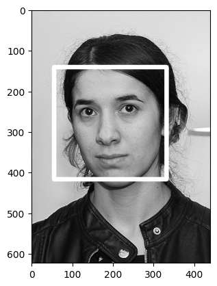
26 人脸检测(Face Detection)
这里是检测有没有人脸,不是识别,用的是cv的传统方法
import numpy as np
import cv2
import matplotlib.pyplot as plt

nadia = cv2.imread('./Nadia_Murad.jpg',0)
denis = cv2.imread('./Denis_Mukwege.jpg',0)
solvay = cv2.imread('./solvay_conference.jpg',0)

face_cascade = cv2.CascadeClassifier('./haarcascade_frontalface_default.xml')

def detect_face(img):


    face_img = img.copy()

    face_rects = face_cascade.detectMultiScale(face_img)

    for (x,y,w,h) in face_rects:
        cv2.rectangle(face_img, (x,y), (x+w,y+h), (255,255,255), 10)

    return face_img

result = detect_face(nadia)
plt.imshow(result,cmap='gray')
在摄像头 / 视频上检测
cap = cv2.VideoCapture(0)

while True:

    ret, frame = cap.read(0)

    frame = detect_face(frame)

    cv2.imshow('Video Face Detection', frame)

    c = cv2.waitKey(1)
    if c == 27:
        break

cap.release()
cv2.destroyAllWindows()
27 光流(Optical Flow)
GitHub Copilot: 在计算机视觉中,光流(Optical Flow)是指在连续的两帧图像中,同一物体上的像素在时间上的变化量。光流可以用来描述物体的运动,是计算机视觉中的一个重要问题。
光流算法可以通过比较相邻帧之间的像素强度值来计算像素的运动。具体来说,它会在第一帧中选择一个像素,然后在第二帧中找到与该像素最相似的像素,并计算它们之间的位移量。这个过程会对图像中的每个像素进行,从而得到整个图像的光流场。
光流算法可以用于许多计算机视觉应用,例如运动跟踪、视频稳定和人体姿态估计等。
nextPts, status, err = cv2.calcOpticalFlowPyrLK(prev_gray, frame_gray, prevPts, None, **lk_params)

flow = cv2.calcOpticalFlowFarneback(prvsImg,nextImg, None, 0.5, 3, 15, 3, 5, 1.2, 0)
28 MeanShift目标追踪(MeanShift Tracking)
在计算机视觉中,MeanShift Tracking是一种目标跟踪算法,用于在视频序列中跟踪运动的目标。它基于颜色直方图的密度估计方法,可以自适应地调整目标区域的大小和形状,以适应目标的运动和变化。
MeanShift Tracking算法的基本思想是在当前帧中选择一个初始目标区域,并计算该区域的颜色直方图。然后,它会在下一帧中搜索与该直方图最相似的区域,并将其作为新的目标区域。这个过程会迭代进行,直到目标区域的位置不再发生变化或达到最大迭代次数为止。
# Grab the Frame in HSV
        hsv = cv2.cvtColor(frame, cv2.COLOR_BGR2HSV)

        # Calculate the Back Projection based off the roi_hist created earlier
        dst = cv2.calcBackProject([hsv],[0],roi_hist,[0,180],1)

        # Apply meanshift to get the new coordinates of the rectangle
        ret, track_window = cv2.meanShift(dst, track_window, term_crit)

        # Draw the new rectangle on the image
        x,y,w,h = track_window
        img2 = cv2.rectangle(frame, (x,y), (x+w,y+h), (0,0,255),5)

        cv2.imshow('img2',img2)
29 CamShift目标追踪(CamShift Tracking)
GitHub Copilot: 在计算机视觉中,CamShift Tracking是一种基于MeanShift Tracking算法的改进算法,用于在视频序列中跟踪运动的目标。它可以自适应地调整目标区域的大小和形状,以适应目标的运动和变化,并且可以处理目标的旋转和缩放。
CamShift Tracking算法的基本思想是在当前帧中选择一个初始目标区域,并计算该区域的颜色直方图。然后,它会在下一帧中搜索与该直方图最相似的区域,并将其作为新的目标区域。与MeanShift Tracking算法不同的是,CamShift Tracking算法会根据目标区域的颜色直方图计算目标的中心点和大小,并使用这些信息来调整搜索窗口的大小和形状。这个过程会迭代进行,直到目标区域的位置和大小不再发生变化或达到最大迭代次数为止。
# Grab the Frame in HSV
        hsv = cv2.cvtColor(frame, cv2.COLOR_BGR2HSV)

        # Calculate the Back Projection based off the roi_hist created earlier
        dst = cv2.calcBackProject([hsv],[0],roi_hist,[0,180],1)


        # Apply Camshift to get the new coordinates of the rectangle
        ret, track_window = cv2.CamShift(dst, track_window, term_crit)

        # Draw it on image
        pts = cv2.boxPoints(ret)
        pts = np.int0(pts)
        img2 = cv2.polylines(frame,[pts],True, (0,0,255),5)
        cv2.imshow('img2',img2)
30 其他目标追踪算法
GitHub Copilot: OpenCV中的tracking API提供了多种目标跟踪算法,包括Boosting、MIL、KCF、TLD、MedianFlow、CamShift和MeanShift等。这些算法都是用于在视频序列中跟踪运动的目标,但它们的实现方式和性能特点不同。
其中,CamShift和MeanShift算法是基于颜色直方图的密度估计方法,可以自适应地调整目标区域的大小和形状,以适应目标的运动和变化。CamShift算法是MeanShift算法的改进版,可以处理目标的旋转和缩放。
Boosting、MIL和KCF算法是基于机器学习的目标跟踪算法,使用分类器来区分目标和背景,并根据分类器的输出来更新目标的位置和大小。这些算法通常具有较高的跟踪精度和鲁棒性,但需要较长的训练时间和较高的计算资源。
TLD和MedianFlow算法是基于特征点的目标跟踪算法,使用特征点来描述目标的外观和运动,并根据特征点的位置和运动来更新目标的位置和大小。这些算法通常具有较快的跟踪速度和较好的鲁棒性,但对目标的外观和运动有一定的限制。
在实际应用中,可以根据目标的特点和应用场景选择合适的跟踪算法。例如,对于需要处理目标旋转和缩放的场景,可以选择CamShift算法;对于需要高精度和鲁棒性的场景,可以选择Boosting、MIL或KCF算法;对于需要快速跟踪和鲁棒性的场景,可以选择TLD或MedianFlow算法。